Energy Street · Rod pump diagnostics
Dynamometer card analysis: from the surface card to the pump card and a diagnosis
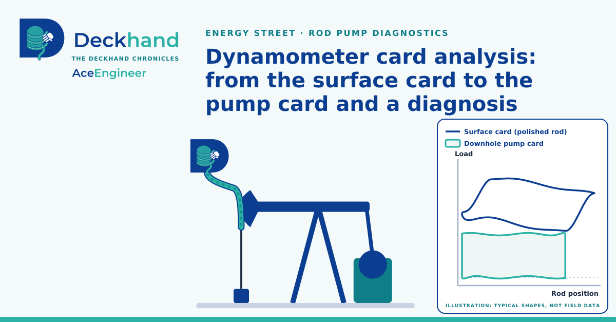
A surface card, measured at the top of a rod-pumped well, carries enough to see the pump at the bottom of the well and to screen that pump from the office.
| Objective | Screen rod pump from the surface card measured at the top of the well. |
|---|---|
| Inputs | The surface card: the load on the polished rod against its position, over one stroke. The well's rod and pump data: rod sizes and lengths, pump depth, plunger size and pumping speed. |
| Method |
|
| Output | The pump card, its stroke, fillage and fluid load, and a first reading of the pump's condition, as a hypothesis to check at the well. |
| Data | A public example well, and ten labelled card shapes of common pump conditions, called a diagnostic plate, from a public rod-pump dataset published on Mendeley Data in 2020 [3]. |
| Result | Example well: the pump moves 73 % of the surface stroke and, on its only card, a shutdown card, fills to 60 %. Ten shapes: the shape model names 6 of 10. |
Diagnosing a rod pump is always a challenge. The pump works at the bottom of the well, out of sight. Some wells measure the downhole card, but most measure only the surface card: the load on the polished rod against its position, over one stroke. The card data contains all of this information at once: the pump's work, the weight, stretch and vibration of the rod string, the pumping unit, even loose bolts, so a pump problem can hide inside it.
Our troubleshooting tool computes the pump card from the surface card and gives a first reading of the pump's condition. To keep the problem simple, it models the rod string only to remove its effect from the card. The rod string, the pumping unit and other component anomalies are the subjects of later articles in this rod pump series, and practical diagnostics and repairs follow the engineering.
- Check a well from the office, and plan the visit around a specific check.
- The more suitable data you give it, with fewer assumptions, the better the pump card and the diagnosis.
- Reusable prompt to try a public example well or perform own data custom investigations.
Some background, for readers who want it. A new well often flows on its own: the reservoir pressure pushes oil, water and gas up the tubing to the surface. As the well produces, the reservoir pressure declines, until it can no longer lift the fluid to the surface. The well then needs artificial lift, a pump or injected gas that adds the energy the reservoir no longer supplies.
The main artificial lift methods are the rod pump, the electric submersible pump, gas lift, the progressing cavity pump, plunger lift and the hydraulic pump; each suits different rates, depths and well conditions. In a rod pump, a pumping unit at the surface strokes a string of steel rods, and the rods drive a plunger pump at the bottom of the well. The surface card records the load on that rod string over each stroke.
Life of a well, schematic: natural flow, reservoir pressure decline and artificial lift. This article deals with the rod pump.
That is the background. The rest of the article works with the rod pump.
Based on public data, the surface card of an example well and the pump card computed from it are shown in Figure 1.
- The blue loop is the surface card, measured at the top of the rod string.
- The orange loop is the pump card computed from it, at the bottom of the 4,750 ft rod string.
- The rods stretch and vibrate, so the 54.0 in surface stroke becomes a 39.6 in stroke at the pump.
- Surface stroke 54.0 in, pump stroke 39.6 in; each card is drawn from the bottom of its stroke.
- Data: figure-1-cards.csv, version of 13 Nov 2026.
Figure 1. The pump moves 73 % of the surface stroke, fills to 60 % and lifts 3,310 lbf: surface and pump cards of the public example well.
Key conclusions
The key conclusions for the example well are as follows:
- On this card the pump fills to 60 % of its stroke (fillage: effective plunger travel as a share of the pump stroke). At this card's fillage, 24 hours a day and no slip, it displaces 40.0 bbl/day, against 66.6 bbl/day for a full pump, so about 27 bbl/day of pump capacity is not used.
- Fillage in normal operation is not established. The only card is a shutdown card, the card the pump controller stores when it stops the pump, and the source system's own corner detection, which finds where the valves open and close, failed on it. Its cause, whether inflow, gas, valve leakage or a corner-detection error, is a check for the well.
- The plunger lifts a fluid load of 3,310 lbf on each upstroke.
- The pump stroke is 39.6 in, 73 % of the surface stroke. Rod stretch and rod dynamics take the rest.
- The shape model, a classifier that gives each of 18 pump conditions a class probability from the card's shape, reads this card as tagging up, the plunger striking at the top of its stroke. The same model missed tagging up in its own ten-example test (Example 5, Figure 2), so this is a weak hypothesis to check at the well. It is independent of the fillage, which comes from the valve points on the pump card, not from the card's shape.
Two numerical methods are available for the pump card: a finite-difference method [2] and a frequency-domain method [1]. On this well their pump cards differ by 0.26 % (root mean square) of the load range, the span from the smallest to the largest load on the card, so for this problem the two methods are equivalent. Appendices A and B give the example well and the comparison.
Pump condition diagnostics from surface cards
Based on public data, ten common pump conditions are run through the same analysis. Each surface card is built from one of the ten labelled card shapes of a public diagnostic plate [3], taken as a pump card by assumption, at an assumed stroke and load, so the cards illustrate shapes rather than field wells. They are shown in Figure 2.
- A round trip through the same rod model recovers every pump card within 0.4 to 2.4 % (root mean square) of its load range: a self-consistency check, not a validation.
- The shape model names 6 of the 10 conditions correctly (5 firm, 1 by name mapping).
- Where it misses, it reads tagging up, tagging down, plunger out of barrel and sand production as a traveling valve leak.
| No. | Condition (plate label) | Model reading | Match | Fillage (%) | Fluid load (lbf) |
|---|---|---|---|---|---|
| 1 | Normal operation | normal operation (81 %) | yes | 84 | 3,711 |
| 2 | Insufficient supply | fluid pound (99 %) | yes, assumed | 23 | 3,020 |
| 3 | Gas interference | gas interference (51 %) | yes | 28 | 3,405 |
| 4 | Rod parting | rod parting (over 99 %) | yes | 92 | 2,935 |
| 5 | Tagging up | traveling valve leak (over 99 %) | no | 70 | 3,456 |
| 6 | Tagging down | traveling valve leak (99 %) | no | 79 | 3,303 |
| 7 | Traveling valve leakage | traveling valve leak (over 99 %) | yes | 94 | 3,403 |
| 8 | Standing valve leakage | standing valve leak (over 99 %) | yes | 74 | 3,762 |
| 9 | Plunger out of barrel | traveling valve leak (62 %) | no | 94 | 2,554 |
| 10 | Sand production | traveling valve leak (over 99 %) | no | 77 | 3,235 |
Example 1: Normal operation
Example 1 is selected in the table. Select another row to show its cards and reading.
Ideal pump, for comparison
Normal operation
- Round trip through the same rod model: 0.5 % (root mean square) of the load range.
- Fillage reads 83.6 % and fluid load 3,711 lbf.
- The shape model reads normal operation (81 %), which matches the plate label.
Example 2: Insufficient supply
Example 2 is selected in the table. Select another row to show its cards and reading.
Ideal pump, for comparison
Insufficient supply
- Round trip through the same rod model: 0.9 % (root mean square) of the load range.
- Fillage reads 23.1 % and fluid load 3,020 lbf.
- The shape model reads fluid pound (99 %), which matches the plate label.
Example 3: Gas interference
Example 3 is selected in the table. Select another row to show its cards and reading.
Ideal pump, for comparison
Gas interference
- Round trip through the same rod model: 0.4 % (root mean square) of the load range.
- Fillage reads 28.3 % and fluid load 3,405 lbf.
- The shape model reads gas interference (51 %), which matches the plate label. The two highest classes are close (51 % and 49 %), so this reading is uncertain.
Example 4: Rod parting
Example 4 is selected in the table. Select another row to show its cards and reading.
Ideal pump, for comparison
Rod parting
- Round trip through the same rod model: 0.6 % (root mean square) of the load range.
- Fillage reads 92.4 % and fluid load 2,935 lbf.
- The shape model reads rod parting (over 99 %), which matches the plate label.
Example 5: Tagging up
Example 5 is selected in the table. Select another row to show its cards and reading.
Ideal pump, for comparison
Tagging up
- Round trip through the same rod model: 0.8 % (root mean square) of the load range.
- Fillage reads 70.2 % and fluid load 3,456 lbf.
- The shape model reads traveling valve leak (over 99 %); the plate label is tagging up.
Example 6: Tagging down
Example 6 is selected in the table. Select another row to show its cards and reading.
Ideal pump, for comparison
Tagging down
- Round trip through the same rod model: 0.4 % (root mean square) of the load range.
- Fillage reads 79.0 % and fluid load 3,303 lbf.
- The shape model reads traveling valve leak (99 %); the plate label is tagging down.
Example 7: Traveling valve leakage
Example 7 is selected in the table. Select another row to show its cards and reading.
Ideal pump, for comparison
Traveling valve leakage
- Round trip through the same rod model: 0.5 % (root mean square) of the load range.
- Fillage reads 93.7 % and fluid load 3,403 lbf.
- The shape model reads traveling valve leak (over 99 %), which matches the plate label.
Example 8: Standing valve leakage
Example 8 is selected in the table. Select another row to show its cards and reading.
Ideal pump, for comparison
Standing valve leakage
- Round trip through the same rod model: 0.5 % (root mean square) of the load range.
- Fillage reads 74.5 % and fluid load 3,762 lbf.
- The shape model reads standing valve leak (over 99 %), which matches the plate label.
Example 9: Plunger out of barrel
Example 9 is selected in the table. Select another row to show its cards and reading.
Ideal pump, for comparison
Plunger out of barrel
- Round trip through the same rod model: 0.5 % (root mean square) of the load range.
- Fillage reads 93.6 % and fluid load 2,554 lbf.
- The shape model reads traveling valve leak (62 %); the plate label is plunger out of barrel.
Example 10: Sand production
Example 10 is selected in the table. Select another row to show its cards and reading.
Ideal pump, for comparison
Sand production
- Round trip through the same rod model: 2.4 % (root mean square) of the load range.
- Fillage reads 77.1 % and fluid load 3,235 lbf.
- The shape model reads traveling valve leak (over 99 %); the plate label is sand production.
- Example 3, gas interference, is selected when the page opens. Pointing at a row also selects it; the arrow keys move between rows.
- Each panel shows the ideal cards above the cards of the selected condition: the surface card (blue), the plate shape (grey) and the computed pump card (orange), with the shape model's three highest classes. Both charts in a panel share one scale.
- Ideal cards: a textbook ideal pump card, a full pump with no leakage whose valves open and close at the ends of the stroke, is drawn as a rectangle, scaled to the same stroke and load as the plate shapes and lifted to its surface card with the same rod model. It is the same for all ten conditions, because all ten use the same well, stroke and load.
- Run through the same analysis, the ideal card reads a fillage of 96 % and a fluid load of 3,944 lbf, and the shape model reads it as traveling valve leak (over 99 %).
- Match "yes, assumed": the plate label is matched by assumption to a model class of another name.
- Fillage and fluid load come from reference shapes scaled to an assumed stroke and load, so they show the method, not a well; for rod parting they have no physical meaning.
- Data: one CSV per example in the worked examples, version of 14 Nov 2026.
Figure 2. Ten reference card shapes, scaled and run through the analysis, each beside the ideal card: the shape model names 6 of 10. Select a row in the table to show that example.
How the ten examples are built, and the full values, are given in Appendix C.
Run the analysis on measured cards
The same analysis runs in a web page in the digitalmodel library (version of 14 Nov 2026); it needs no installation and no network once its files are on disk. Load a surface card with the well's rod and pump data, and the page draws the pump card and reads fillage, fluid load and the model readings. Its guide gives the file format.
Read the full study (version of 12 Nov 2026)
To try it out or adapt the analysis, see reusable prompt.
The work leaves open the accuracy of the shape model's readings on field cards: it is trained on generated cards, and no labelled field cards were available to test it.
If you have run your own analysis, see a way to improve this one, or have an idea for a future issue, write to support@aceengineer.com. We read every reply and credit the ideas we use and provide results we obtained.
Prepared: Analyst Deckhand · Checked: Editor Deckhand · Approved: Vamsee Achanta · 19 November 2026
References
- Gibbs, S. G. (1963). Predicting the Behavior of Sucker-Rod Pumping Systems. SPE-588-PA. doi:10.2118/588-PA.
- Everitt, T. A. and Jennings, J. W. (1992). An Improved Finite-Difference Calculation of Downhole Dynamometer Cards for Sucker-Rod Pumps. SPE-18189-PA. doi:10.2118/18189-PA.
- Zhang, R. (2020). Data for: Real time and intelligent diagnosis method of working condition in rod pumping well based on multi-dimensional data coupling of reservoir-wellbore-surface. Mendeley Data, version 1, CC0 1.0. Diagnostic plate of ten pump working conditions. doi:10.17632/hnfwm9mjs6.1, retrieved 11 Oct 2026.
- digitalmodel library, MIT licence, version of 14 Nov 2026. github.com/vamseeachanta/digitalmodel.
Appendix A Example well: inputs, results and limits
The example well behind Figure 1 and the key conclusions is summarised in this appendix.
- The well is one anonymised field well in the digitalmodel library: a 1.500 in plunger at 4,844 ft on a two-taper steel rod string, pumped at 6.42 strokes a minute.
- The inputs that matter most: a 1 % larger rod diameter lowers the maximum pump load by about 3.2 %, and a 1 % load-cell gain error raises it by about 2.6 %.
- Unanchored tubing is not modelled and only steel rods are accepted. Both methods and the web page treat the well as vertical; a deviation survey is flagged, not modelled.
Inputs, results, sensitivity and limits in full: digitalmodel on GitHub, example-well.md.
Appendix B The two numerical methods compared
The key conclusion of the comparison of the two methods is given in this appendix.
- A finite-difference method [2], the default, and a frequency-domain method [1] compute the pump card. On the example well their pump cards differ by 0.26 % (root mean square) of the load range, and each differs from the card stored in the well record by at most 0.78 %.
- For this problem, at this accuracy, the methods are equivalent. All results in this article use the default method.
- As more types of card come in, the two methods are kept side by side: some physical behaviour may be captured better by one method than by the other.
Methods and comparison in full: digitalmodel on GitHub, numerical-methods.md.
Appendix C The ten examples in detail
How the ten examples of Figure 2 are built is summarised in this appendix.
- Each surface card starts from one of the ten shapes of the public diagnostic plate [3], taken as a pump card by assumption and scaled to an assumed stroke and load. It is lifted to the surface through the rod string of the example well and then analysed like a measured card.
- The web page gives the same results as the library on all ten examples: the same model labels, and pump loads that differ by at most 3 × 10⁻⁹ lbf, a rounding-level difference.
Basis, assumptions and the full values of each example: digitalmodel on GitHub, ten-examples.md.
Appendix D Reusable prompts
- Rebuild this analysis from public code with your own assistant, and check it against the published values.
- Then run it on a surface card of your own well.
Prompts, data and check values: digitalmodel on GitHub, reusable-prompts.md.
Public data set: the example well, file cleansed_well_001.json of the digitalmodel library, MIT licence, version of 14 Nov 2026; the diagnostic plate [3], CC0 1.0, retrieved 11 Oct 2026.